Data model

Defining the data model is a crucial step before training one of getML's Pipelines. You typically deal with this step after having imported your data and specified the roles of each column.

When working with getML, the raw data usually comes in the form of relational data. That means the information relevant for a prediction is spread over several tables. The data model is the definition of the relationships between all of them.

Most relational machine learning problems can be represented in the form of a star schema, in which case you can use the StarSchema abstraction. If your dataset is a time series, you can use the TimeSeries abstraction.

Tables

The population table

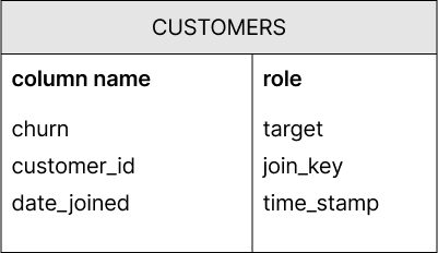
The population table is the main table of the analysis. It defines the statistical population of your machine learning problem and contains the target variable(s), which we want to predict. Furthermore, the table usually also contains one or more columns with the role join_key. These are keys used to establish a relationship – also called joins – with one or more peripheral tables.

The example below contains the population table of a customer churn analysis. The target variable is churn – whether a person stops using the services and products of a company. It also contains the information whether or not a given customer has churned after a certain reference date. The join key customer_id is used to establish relations with a peripheral table. Additionally, the date the customer joined the company is contained in the column date_joined, which we have assigned the role time_stamp.

Peripheral tables

Peripheral tables contain additional information relevant for the prediction of the target variable in the population table. Each of them is related to the latter (or another peripheral table, refer to the snowflake schema) via a join_key.

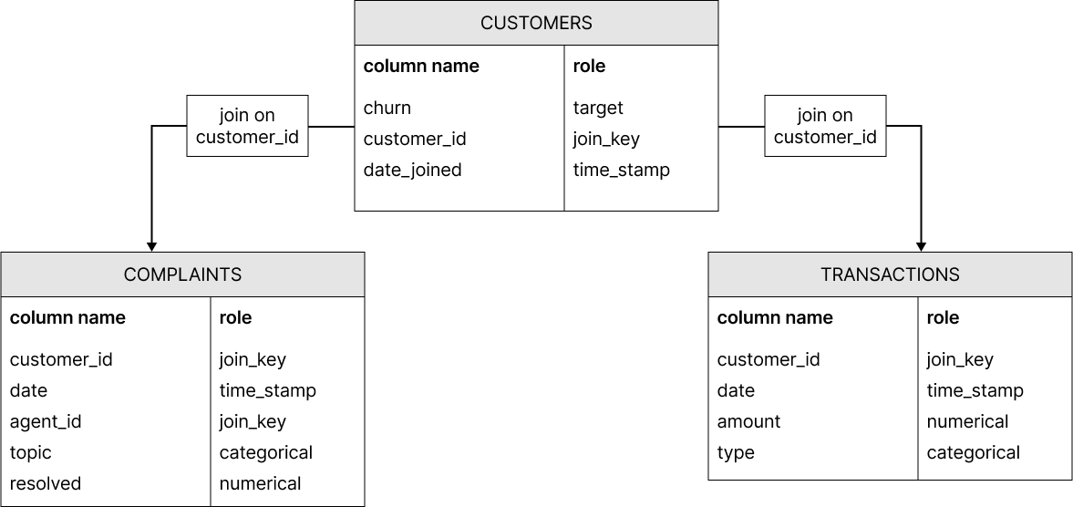
The images below represent two peripheral tables that could be used for our customer churn analysis. One table represents complaints a customer made with a certain agent, and the other represents the transactions the customer made using their account.

Placeholders

In getML, Placeholders are used to construct the DataModel. They are abstract representations of DataFrames or Views and the relationships among each other, but do not contain any data themselves.

The idea behind the placeholder concept is that they allow constructing an abstract data model without any reference to an actual dataset. This data model serves as input for the Pipeline. Later on, the feature_learning algorithms can be trained and applied on any dataset that follows this data model.

More information on how to construct placeholders and build a data model can be found in the API documentation for Placeholder and DataModel.

Joins

Joins are used to establish relationships between placeholders. To join two placeholders, the data frames used to derive them should both have at least one join_key. The joining itself is done using the join() method (follow the link for examples).

All columns corresponding to time stamps have to be given the role time_stamp, and one of them in both the population and peripheral table is usually passed to the join() method. This approach ensures that no information from the future is considered during training by including only those rows of the peripheral table in the join operation for which the time stamp of the corresponding row in the population table is either the same or more recent.

Data schemata

After creating placeholders for all data frames in an analysis, we are ready to create the actual data schema. A data schema is a certain way of assembling population and peripheral tables.

The star schema

The StarSchema is the simplest way of establishing relations between the population and the peripheral tables, sufficient for the majority of data science projects.

In the star schema, the population table is surrounded by any number of peripheral tables, all joined via a certain join key. However, no joins between peripheral tables are allowed.

Because this is a very popular schema in many machine learning problems on relational data, getML contains a special class for these sorts of problems: StarSchema.

The population table and two peripheral tables introduced in Tables can be arranged in a star schema like this:

The snowflake schema

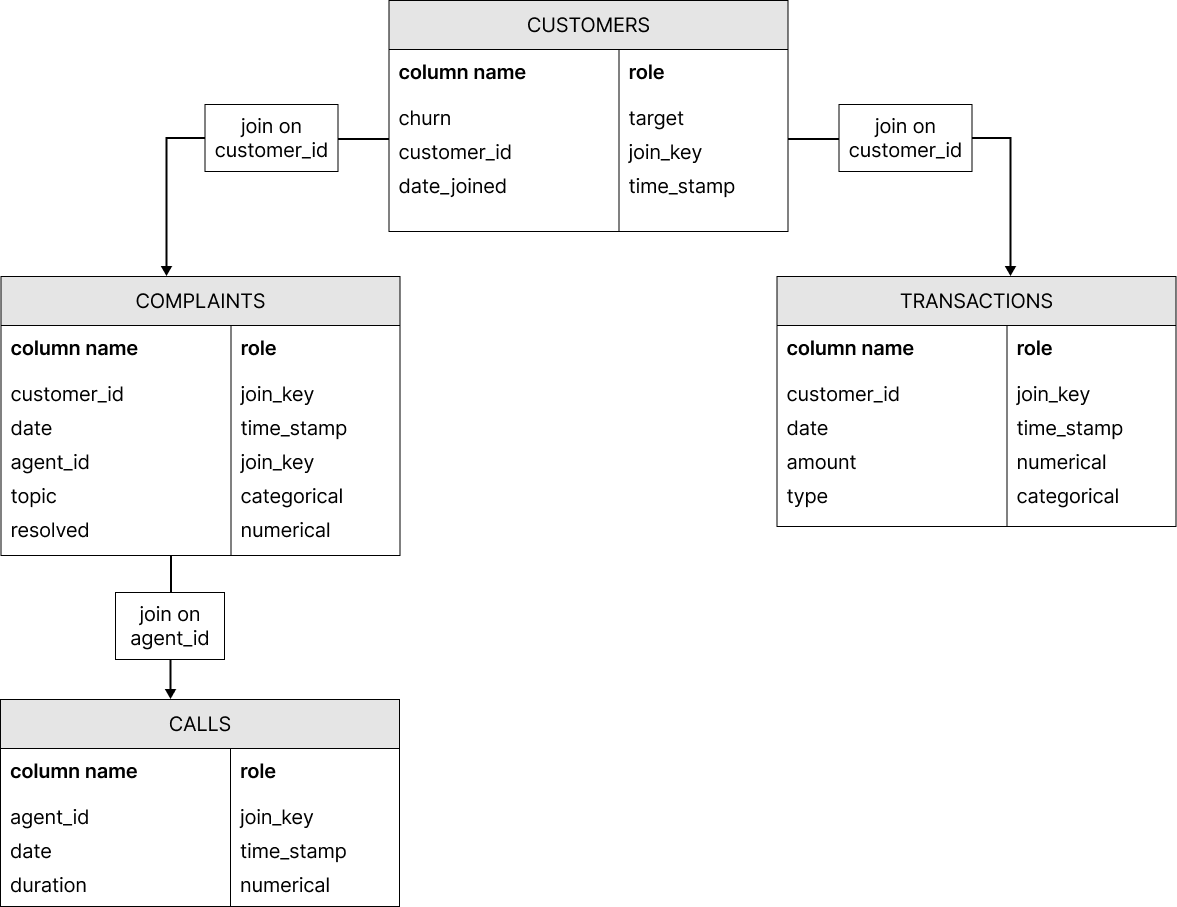
In some cases, the star schema is not enough to represent the complexity of a dataset. This is where the snowflake schema comes in: In a snowflake schema, peripheral tables can have peripheral tables of their own.

Assume that in the customer churn analysis shown earlier, there is an additional table containing information about the calls a certain agent made in customer service. It can be joined to the COMPLAINTS table using the key agent_id.

To model snowflake schemata, you need to use the DataModel and Container classes.

Time series

Time series can be handled by a self-join. In addition, some extra parameters and considerations are required when building features based on time stamps.

Self-joining a single table

If you are dealing with a classical (multivariate) time series and all your data is contained in a single table, all the concepts covered so far still apply. You just have to perform a so-called self-join by providing your table as both the population and peripheral table and join them.

The process works as follows: Whenever a row in the population table - a single measurement - is taken, it will be combined with all the content of the peripheral table - the same time series - for which the time stamps are smaller than the one in the line we picked. A familiar term for this is a "rolling window".

You can also use the TimeSeries abstraction, which abstracts away the self-join. In this case, you do not have to think about self-joins too much.

Horizon and Memory

Crucial concepts of time series analysis are horizon and memory. In the context of getML's time series analysis, horizon is defined as a point forecast. That means the prediction of the target variable at the point as far in the future as defined by the horizon.

Memory, on the other hand is the time duration into the past, that is considered when making a prediction. The memory is used to define the time window of data entering the model between the past and now. The horizon defines the point in the future that the predictions is being made for.

time_stamps and on

Two parameters in the time series signature determine how the self join is carried out. The time_stamps parameter defines what column is the underlying time dimension to which memory and horizon are applied to. The chosen column must also be of role time_stamp.

on simply provides an extra handle to control, what subset of the data is part of any given time series. For example if you have a time series of sales data, you might want to only consider the sales data of a certain product category. In this case you would specify the on parameter to be the column containing the product category.

Lagged Target and horizon

Another useful parameter in time series analysis is lagged_target. This boolean controls whether the target variable is used as a predictor. Including the target variable as a predictor can be useful in time series analysis, when at time of prediction, the target variable up until and including now is known. In turn, this means lagged target variables are only permissible if the target variable is predicted for some when in the future. That is, the horizon must be assigned a positive value.

Features based on time stamps

The getML Engine is able to automatically generate features based on aggregations over time windows. Both the length of the time window and the aggregation itself will be determined by the feature learning algorithm. The only requirement is to provide the temporal resolution your time series is sampled with in the delta_t parameter in any feature learning algorithm.